# Remove input cells at runtime (nbsphinx)
import IPython.core.display as d
d.display_html('<script>jQuery(function() {if (jQuery("body.notebook_app").length == 0) { jQuery(".input_area").toggle(); jQuery(".prompt").toggle();}});</script>', raw=True)

Direction recontruction (DL2)

WARNING

This is still a work-in-progress, it will evolve with the pipeline comparisons and converge with ctaplot+cta-benchmarks.

Author(s):

• Dr. Michele Peresano (CEA-Saclay/IRFU/DAp/LEPCHE), 2020

based on previous work by J. Lefacheur.

Description:

This notebook contains benchmarks for the protopipe pipeline regarding the angular distribution of the showers selected for DL3 data.

NOTES:

• a more general set of benchmarks is being defined in cta-benchmarks/ctaplot,

• follow this document by adding new benchmarks or proposing new ones.

Requirements:

To run this notebook you will need a set of DL2 data produced on the grid with protopipe. The MC production to be used and the appropriate set of files to use for this notebook can be found here.

The data format required to run the notebook is the current one used by protopipe . Later on it will be the same as in ctapipe + pyirf.

Development and testing:

As with any other part of protopipe and being part of the official repository, this notebook can be further developed by any interested contributor.

The execution of this notebook is not currently automatic, it must be done locally by the user - preferably before pushing a pull-request.

IMPORTANT: Please, if you wish to contribute to this notebook, before pushing anything to your branch (better even before opening the PR) clear all the output and remove any local directory paths that you used for testing (leave empty strings).

TODO:

• add missing benchmarks from CTA-MARS comparison

• crosscheck with EventDisplay

Table of contents

• Energy-dependent offset distribution

• Angular resolution

• PSF asymmetry

• True energy distributions

%matplotlib inline
import matplotlib.pyplot as plt
cmap = dict()
import matplotlib.colors as colors
from matplotlib.colors import LogNorm, PowerNorm
count = 0
for key in colors.cnames:
    if 'dark' in key:
    #if key in key:
        cmap[count] = key
        count = count + 1
#cmap = {'black': 0, 'red': 1, 'blue': 2, 'green': 3}
cmap = {0: 'black', 1: 'red', 2: 'blue', 3: 'green'}
import os
from pathlib import Path
import numpy as np
import pandas as pd

import astropy.coordinates as c
import astropy.wcs as wcs
import astropy.units as u
import matplotlib.pyplot as plt

def compute_psf(data, ebins, radius):
    nbin = len(ebins) - 1
    psf = np.zeros(nbin)
    psf_err = np.zeros(nbin)
    for idx in range(nbin):
        emin = ebins[idx]
        emax = ebins[idx+1]
        sel = data.loc[(data['true_energy'] >= emin) & (data['true_energy'] < emax), ['xi']]
        if len(sel) != 0:
            psf[idx] = np.percentile(sel['xi'], radius)
            psf_err[idx] = psf[idx] / np.sqrt(len(sel))
        else:
            psf[idx] = 0.
            psf_err[idx] = 0.
    return psf, psf_err

def plot_psf(ax, x, y, err, **kwargs):
    color = kwargs.get('color', 'red')
    label = kwargs.get('label', '')
    xlabel = kwargs.get('xlabel', '')
    xlim = kwargs.get('xlim', None)

    ax.errorbar(x, y, yerr=err, fmt='o', label=label, color=color) #, yerr=err, fmt='o') #, color=color, label=label)
    ax.set_ylabel('PSF (68% containment)')
    ax.set_xlabel('True energy [TeV]')
    if xlim is not None:
        ax.set_xlim(xlim)
    return ax

# First we check if a _plots_ folder exists already.
# If not, we create it.
Path("./plots").mkdir(parents=True, exist_ok=True)

# EDIT ONLY THIS CELL WITH YOUR LOCAL SETUP INFORMATION
parentDir = "" # full path location to 'shared_folder'
analysisName = ""

indir = os.path.join(parentDir, "shared_folder/analyses", analysisName, "data/DL2")
infile = 'DL2_tail_gamma_merged.h5'
data_evt = pd.read_hdf(os.path.join(indir, infile), "/reco_events")
good_events = data_evt[(data_evt["is_valid"]==True) & (data_evt["NTels_reco"] >= 2) & (data_evt["gammaness"] >= 0.75)]

Here we use events with the following cuts: - valid reconstructed events - at least 2 reconstructed images, regardless of the camera - gammaness > 0.75 (mostly a conservative choice)

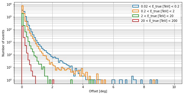
Energy-dependent offset distribution

min_true_energy = [0.02, 0.2, 2, 20]
max_true_energy = [0.2, 2, 20, 200]

plt.figure(figsize=(10,5))
plt.xlabel("Offset [deg]")
plt.ylabel("Number of events")

for low_E, high_E in zip(min_true_energy, max_true_energy):

    selected_events = good_events[(good_events["true_energy"]>low_E) & (good_events["true_energy"]<high_E)]

    plt.hist(selected_events["offset"],
             bins=100,
             range = [0,10],
             label=f"{low_E} < E_true [TeV] < {high_E}",
             histtype="step",
             linewidth=2)

plt.yscale("log")
plt.legend(loc="best")
plt.grid(which="both")

plt.savefig(f"./plots/DL3_offsets_{analysisName}.png")

plt.show()

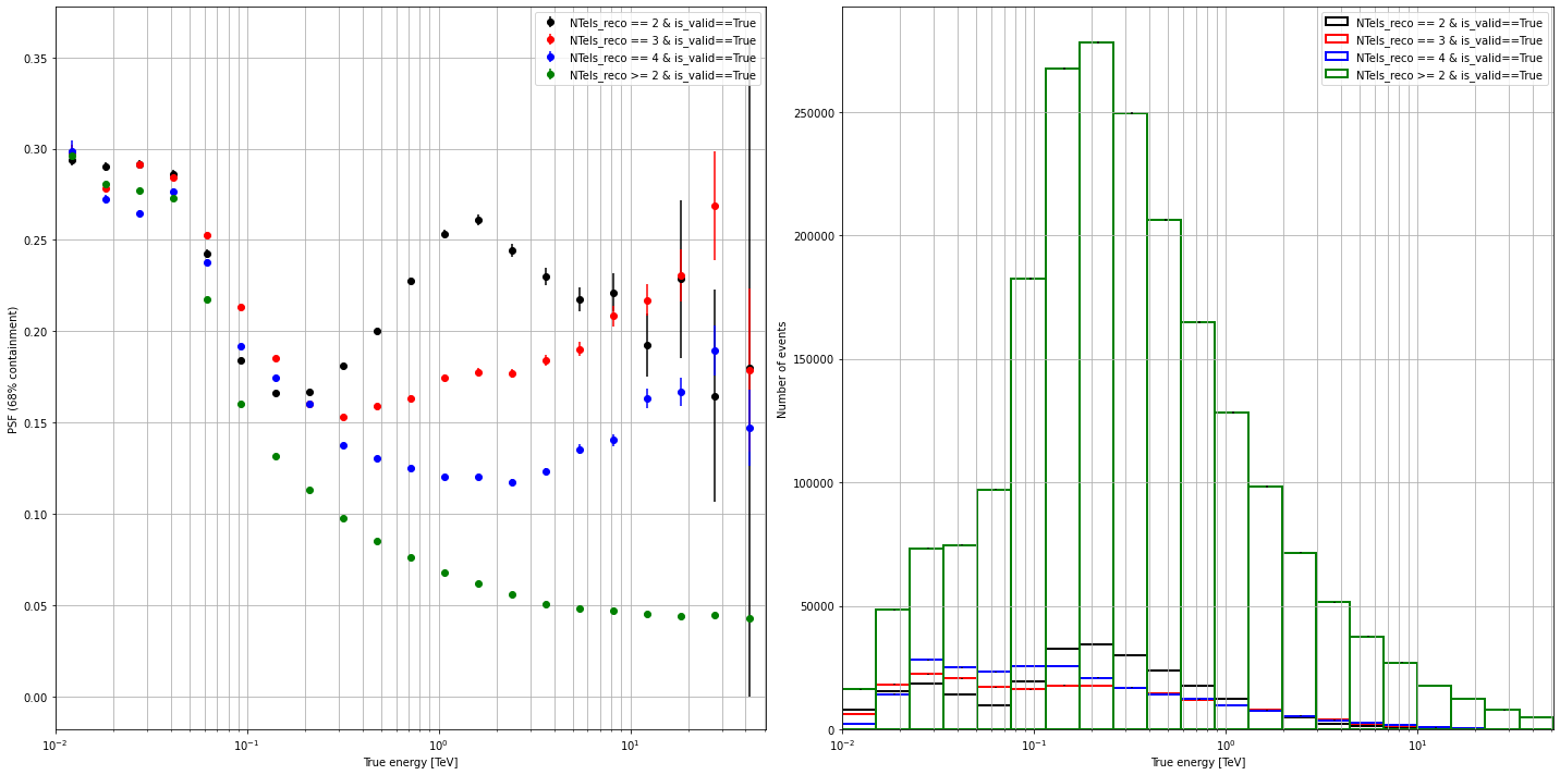
Angular resolution

back to top

Here we compare how the multiplicity influences the performance of reconstructed events.

r_containment = 68

energy_bins = 21
max_energy_TeV = 0.0125
min_energy_TeV = 200.0
energy_edges = np.logspace(np.log10(0.01), np.log10(51), energy_bins + 1, True)
energy = np.sqrt(energy_edges[1:] * energy_edges[:-1])
multiplicity_cuts = ['NTels_reco == 2 & is_valid==True',
                     'NTels_reco == 3 & is_valid==True',
                     'NTels_reco == 4 & is_valid==True',
                     'NTels_reco >= 2 & is_valid==True']

events_selected_multiplicity = [good_events[(good_events["NTels_reco"]==2)],
                                good_events[(good_events["NTels_reco"]==3)],
                                good_events[(good_events["NTels_reco"]==4)],
                                good_events[(good_events["NTels_reco"]>=2)]]

fig, axes = plt.subplots(nrows=1, ncols=2, figsize=(20, 10))
axes = axes.flatten()

cmap = {0: 'black', 1: 'red', 2: 'blue', 3: 'green'}

limit = [0.01, 51]
for cut_idx, cut in enumerate(multiplicity_cuts):
    #data_mult = data_evt.query(cut)
    data_mult = events_selected_multiplicity[cut_idx]
    psf, err_psf = compute_psf(data_mult, energy_edges, 68)
    opt={'color': cmap[cut_idx], 'label': multiplicity_cuts[cut_idx]}
    plot_psf(axes[0], energy, psf, err_psf, **opt)

    y, tmp = np.histogram(data_mult['true_energy'], bins=energy_edges)
    weights = np.ones_like(y)
    #weights = weights / float(np.sum(y))
    yerr = np.sqrt(y) * weights
    centers = 0.5 * (energy_edges[1:] + energy_edges[:-1])
    width = energy_edges[1:] - energy_edges[:-1]
    axes[1].bar(centers, y * weights, width=width, yerr=yerr, **{'edgecolor': cmap[cut_idx], 'label': multiplicity_cuts[cut_idx], 'lw': 2, 'fill': False})
    axes[1].set_ylabel('Number of events')

for ax in axes:
    ax.set_xlim(limit)
    ax.set_xscale('log')
    ax.legend(loc='best')
    ax.grid(which='both')
    ax.set_xlabel('True energy [TeV]')

plt.tight_layout()

fig.savefig(f"./plots/DL3_PSF_{analysisName}.png")

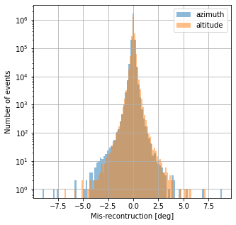
PSF asymmetry

back to top

reco_alt = good_events.reco_alt
reco_az = good_events.reco_az

# right now all reco_az for a 180° deg simualtion turn out to be all around -180°
#if ~np.count_nonzero(np.sign(reco_az) + 1):
reco_az = np.abs(reco_az)

# this is needed for projecting the angle onto the sky
reco_az_corr = reco_az * np.cos(np.deg2rad(good_events.reco_alt))

true_alt = good_events.iloc[0].true_alt
true_az = good_events.iloc[0].true_az

daz = reco_az - true_az
daz_corr = daz * np.cos(np.deg2rad(reco_alt))
dalt = reco_alt - true_alt

plt.figure(figsize=(5, 5))

plt.xlabel("Mis-recontruction [deg]")
plt.ylabel("Number of events")

plt.hist(daz_corr, bins=100, alpha=0.5, label = "azimuth")
plt.hist(dalt, bins=100, alpha=0.5, label = "altitude")

plt.legend()
plt.yscale("log")
plt.grid()

print("Mean and STDs of sky-projected mis-reconstruction axes")
print('daz = {:.4f} +/- {:.4f} deg'.format(daz_corr.mean(), daz_corr.std()))
print('dalt = {:.4f} +/- {:.4f} deg'.format(dalt.mean(), dalt.std()))

plt.show()

Mean and STDs of sky-projected mis-reconstruction axes
daz = -0.0070 +/- 0.1190 deg
dalt = 0.0003 +/- 0.1429 deg

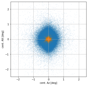
2D representation with orange events being those with offset < 1 deg and E_true > 20 TeV

angcut = (good_events['offset'] < 1) & (good_events['true_energy'] > 20)

plt.figure(figsize=(5,5))
ax = plt.gca()
FOV_size = 2.5 # deg

ax.scatter(daz_corr, dalt, alpha=0.1, s=1, label='no angular cut')
ax.scatter(daz_corr[angcut], dalt[angcut], alpha=0.05, s=1, label='offset < 1 deg & E_true > 20 TeV')

ax.set_aspect('equal')
ax.set_xlabel('cent. Az [deg]')
ax.set_ylabel('cent. Alt [deg]')
ax.set_xlim(-FOV_size,FOV_size)
ax.set_ylim(-FOV_size,FOV_size)
plt.tight_layout()
plt.grid(which="both")

fig.savefig(f"./plots/PSFasymmetry_2D_altaz_{analysisName}.png")

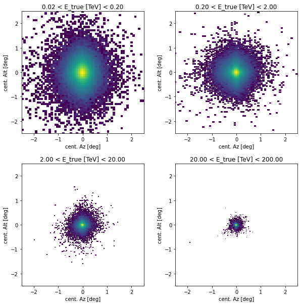
True energy distributions

back to top

plt.figure(figsize=(10,10))
plt.subplots_adjust(hspace=0.25)
true_energy_bin_edges = np.logspace(np.log10(0.02), np.log10(200), 5)
nbins = 200

for i in range(len(true_energy_bin_edges)-1):

    plt.subplot(2, 2, i+1)

    mask = (good_events["true_energy"]>true_energy_bin_edges[i]) & (good_events["true_energy"]<true_energy_bin_edges[i+1])

    plt.hist2d(daz_corr[mask], dalt[mask], bins=[nbins,nbins], norm=LogNorm())
    plt.gca().set_aspect('equal')
    #plt.colorbar()
    plt.xlim(-FOV_size, FOV_size)
    plt.ylim(-FOV_size, FOV_size)
    plt.title(f"{true_energy_bin_edges[i]:.2f} < E_true [TeV] < {true_energy_bin_edges[i+1]:.2f}")
    plt.xlabel('cent. Az [deg]')
    plt.ylabel('cent. Alt [deg]')