# Remove input cells at runtime (nbsphinx)
import IPython.core.display as d
d.display_html('<script>jQuery(function() {if (jQuery("body.notebook_app").length == 0) { jQuery(".input_area").toggle(); jQuery(".prompt").toggle();}});</script>', raw=True)

Particle classification (DL2)

Author(s):

• Dr. Michele Peresano (CEA-Saclay/IRFU/DAp/LEPCHE), 2020

based on previous work by J. Lefacheur.

Description:

This notebook contains benchmarks for the protopipe pipeline regarding particle classification at the DL2 level. The plots shown here are performed also by protopipe.scripts.model_diagnostics which will be discontinued.

NOTES: - these benchmarks will be cross-validated and migrated in cta-benchmarks/ctaplot, - follow this document by adding new benchmarks or proposing new ones.

Requirements:

To run this notebook you will 1 merged files of DL2 data per particle type produced on the grid with protopipe.

When comparing the performance of protopipe with that of CTAMARS (2019), the MC production to be used and the appropriate set of files to use for this notebook can be found here.

The data format required to run the notebook is the current one used by protopipe .

Development and testing:

As with any other part of protopipe and being part of the official repository, this notebook can be further developed by any interested contributor.

The execution of this notebook is not currently automatic: it must be done locally by the user - preferably before pushing a pull-request.

Please, if you wish to contribute to this notebook, before pushing clear all the output and remove local directory paths (leave empty strings).

TODO:

* check any missing model diagnostics product * add remaining benchmarks from CTA-MARS comparison * same for EventDisplay

Table of contents

• Estimate distribution

• ROC curve

%matplotlib inline
import os
from pathlib import Path
import yaml
import matplotlib.pyplot as plt
import pandas as pd
import numpy as np
from sklearn.metrics import auc, roc_curve

def load_config(name):
    """Load YAML configuration file."""
    try:
        with open(name, "r") as stream:
            cfg = yaml.load(stream, Loader=yaml.FullLoader)
    except FileNotFoundError as e:
        print(e)
        raise
    return cfg

def plot_hist(ax, data, nbin, limit, norm=False, yerr=False, hist_kwargs={}, error_kw={}):
    """Utility function to plot histogram"""
    bin_edges = np.linspace(limit[0], limit[-1], nbin + 1, True)
    y, tmp = np.histogram(data, bins=bin_edges)
    weights = np.ones_like(y)
    if norm is True:
        weights = weights / float(np.sum(y))
    if yerr is True:
        yerr = np.sqrt(y) * weights
    else:
        yerr = np.zeros(len(y))

    centers = 0.5 * (bin_edges[1:] + bin_edges[:-1])
    width = bin_edges[1:] - bin_edges[:-1]
    ax.bar(centers, y * weights, width=width, yerr=yerr, error_kw=error_kw, **hist_kwargs)

    return ax

def plot_roc_curve(ax, model_output, y, **kwargs):
    """Plot ROC curve for a given set of model outputs and labels"""
    fpr, tpr, _ = roc_curve(y_score=model_output, y_true=y)
    roc_auc = auc(fpr, tpr)
    label = '{} (area={:.2f})'.format(kwargs.pop('label'), roc_auc)  # Remove label
    ax.plot(fpr, tpr, label=label, **kwargs)
    return ax

def plot_evt_roc_curve_variation(ax, data_test, cut_list, model_output_name):
    """

    Parameters
    ----------
    ax: `~matplotlib.axes.Axes`
        Axis
    data_test: `~pd.DataFrame`
        Test data
    cut_list: `list`
         Cut list

    Returns
    -------
    ax:  `~matplotlib.axes.Axes`
        Axis
    """
    color = 1.
    step_color = 1. / (len(cut_list))
    for i, cut in enumerate(cut_list):
        c = color - (i + 1) * step_color

        data = data_test.query(cut)
        if len(data) == 0:
            continue

        opt = dict(color=str(c), lw=2, label='{}'.format(cut.replace('reco_energy', 'E')))
        plot_roc_curve(ax, data[model_output_name], data['label'], **opt)
    ax.plot([0, 1], [0, 1], color='navy', lw=2, linestyle='--')

    return ax

# First we check if a _plots_ folder exists already.
# If not, we create it.
Path("./plots").mkdir(parents=True, exist_ok=True)

# EDIT ONLY THIS CELL WITH YOUR SETUP INFORMATION
parentDir = "" # path to 'shared_folder'
analysisName = ""

configuration = os.path.join(parentDir,
                             "shared_folder/analyses",
                             analysisName,
                             "configs/classifier.yaml")
cfg = load_config(configuration)

if cfg["Method"]["use_proba"] is True:
    model_output = 'gammaness'
    output_range = [0, 1]
else:
    model_output = 'score'
    output_range = [-1, 1]

indir = os.path.join(parentDir,
                     "shared_folder/analyses",
                     analysisName,
                     "data/DL2")

data_gamma = pd.read_hdf(os.path.join(indir, 'DL2_tail_gamma_merged.h5'), "/reco_events").query('NTels_reco >= 2')
data_electron = pd.read_hdf(os.path.join(indir, 'DL2_tail_electron_merged.h5'), "/reco_events").query('NTels_reco >= 2')
data_proton = pd.read_hdf(os.path.join(indir, 'DL2_tail_proton_merged.h5'), "/reco_events").query('NTels_reco >= 2')

data_gamma['label'] = np.ones(len(data_gamma))
data_electron['label'] = np.zeros(len(data_electron))
data_proton['label'] = np.zeros(len(data_proton))

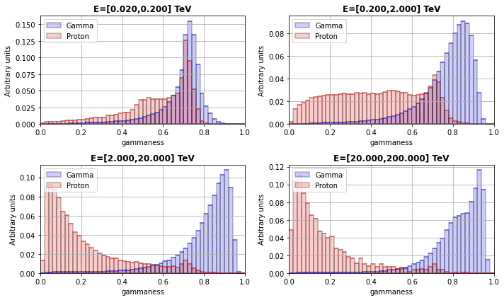
Estimate distribution

back to top

energy_bounds = np.logspace(np.log10(cfg["Diagnostic"]["energy"]["min"]),
                            np.log10(cfg["Diagnostic"]["energy"]["max"]),
                            cfg["Diagnostic"]["energy"]["nbins"] + 1)
ncols = int(cfg["Diagnostic"]["energy"]["nbins"] / 2)
n_ax = len(energy_bounds) - 1
nrows = int(n_ax / ncols) if n_ax % ncols == 0 else int((n_ax + 1) / ncols)
nrows = nrows

fig, axes = plt.subplots(nrows=nrows, ncols=ncols, figsize=(5 * ncols, 3 * nrows))
if nrows == 1 and ncols == 1:
    axes = [axes]
else:
    axes = axes.flatten()

for idx in range(len(energy_bounds) - 1):
    ax = axes[idx]

    # Data selection
    query = 'true_energy >= {} and true_energy < {}'.format(energy_bounds[idx], energy_bounds[idx + 1])
    gamma = data_gamma.query(query)
    proton = data_proton.query(query + ' and offset < {}'.format(1.))
    electron = data_electron.query(query + ' and offset < {}'.format(1.))
    data_list = [gamma, proton]

    # Graphical stuff
    color_list = ['blue', 'red', 'green']
    edgecolor_list = ['black', 'black', 'green']
    fill_list = [True, True, False]
    ls_list = ['-', '-', '--']
    lw_list = [2, 2, 2]
    alpha_list = [0.2, 0.2, 1]
    label_list = ['Gamma', 'Proton', 'Electron']

    opt_list = []
    err_list = []
    for jdx, data in enumerate(data_list):
        opt_list.append(dict(edgecolor=edgecolor_list[jdx], color=color_list[jdx], fill=fill_list[jdx], ls=ls_list[jdx], lw=lw_list[jdx], alpha=alpha_list[jdx], label=label_list[jdx]))
        err_list.append(dict(ecolor=color_list[jdx], lw=lw_list[jdx], alpha=alpha_list[jdx], capsize=3, capthick=2,))

    for jdx, data in enumerate(data_list):
        ax = plot_hist(
            ax=ax, data=data[model_output], nbin=50, limit=output_range,
            norm=True, yerr=False,
            hist_kwargs=opt_list[jdx],
            error_kw=err_list[jdx],
        )
    ax.set_title('E=[{:.3f},{:.3f}] TeV'.format(energy_bounds[idx], energy_bounds[idx + 1]), fontdict={'weight': 'bold'})
    ax.set_xlabel(model_output)
    ax.set_ylabel('Arbitrary units')
    ax.set_xlim(output_range)
    ax.legend(loc='upper left')
    ax.grid()

plt.tight_layout()

fig.savefig(f"./plots/particle_classification_estimate_distribution_protopipe_{analysisName}.png")

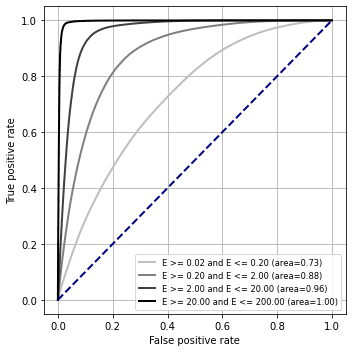
ROC curve

back to top

data = pd.concat([data_gamma, data_electron, data_proton])

plt.figure(figsize=(5,5))

ax = plt.gca()

cut_list = ['reco_energy >= {:.2f} and reco_energy <= {:.2f}'.format(
    energy_bounds[i],
    energy_bounds[i+1]
) for i in range(len(energy_bounds) - 1)]

plot_evt_roc_curve_variation(ax, data, cut_list, model_output)

ax.legend(loc='lower right', fontsize='small')
ax.set_xlabel('False positive rate')
ax.set_ylabel('True positive rate')
ax.grid()
plt.tight_layout()

fig.savefig(f"./plots/particle_classification_roc_curve_protopipe_{analysisName}.png")