[1]:
# Remove input cells at runtime (nbsphinx)
import IPython.core.display as d
d.display_html('<script>jQuery(function() {if (jQuery("body.notebook_app").length == 0) { jQuery(".input_area").toggle(); jQuery(".prompt").toggle();}});</script>', raw=True)
Energy reconstruction (MODEL)
This notebook contains the same code as in protopipe.scripts.model_diagnostic. It should be used to test the performance of the trained model before use it to estimate the energy of DL2 events.
In fact, what happens in a protopipe analysis is that part of the TRAINING sample is used for testing the models to get some preliminary diagnostics. This notebook shows this camera-wise preliminary diagnostics.
Settings and setup of the plots are done using the same configuration file used for training the model.
Developers
Please, if you have any contribution regarding this part, do it here and not in the relevant sections of the main code, which are now discontinued.
Table of contents
[2]:
import gzip
import glob
from os import path

import pickle
import joblib
import yaml
import numpy as np
import pandas as pd
from scipy.optimize import curve_fit

import matplotlib.pyplot as plt
import matplotlib.patches as mpatches
plt.rcParams.update({'figure.max_open_warning': 0})
[3]:
def load_config(name):
    """Load YAML configuration file."""
    try:
        with open(name, "r") as stream:
            cfg = yaml.load(stream, Loader=yaml.FullLoader)
    except FileNotFoundError as e:
        print(e)
        raise
    return cfg
[4]:
def load_obj(name ):
    """Load object in binary"""
    with gzip.open(name, 'rb') as f:
        return pickle.load(f)
[5]:
def plot_hist(ax, data, nbin, limit, norm=False, yerr=False, hist_kwargs={}, error_kw={}):
    """Utility function to plot histogram"""
    bin_edges = np.linspace(limit[0], limit[-1], nbin + 1, True)
    y, tmp = np.histogram(data, bins=bin_edges)
    weights = np.ones_like(y)
    if norm is True:
        weights = weights / float(np.sum(y))
    if yerr is True:
        yerr = np.sqrt(y) * weights
    else:
        yerr = np.zeros(len(y))

    centers = 0.5 * (bin_edges[1:] + bin_edges[:-1])
    width = bin_edges[1:] - bin_edges[:-1]
    ax.bar(centers, y * weights, width=width, yerr=yerr, error_kw=error_kw, **hist_kwargs)

    return ax
[6]:
def plot_distributions(feature_list,
                       data_list,
                       nbin=30,
                       hist_kwargs_list={},
                       error_kw_list={},
                       ncols=2):
    """Plot feature distributions for several data set. Returns list of axes."""
    n_feature = len(feature_list)
    nrows = int(n_feature / ncols) if n_feature % ncols == 0 else int((n_feature + 1) / ncols)
    fig, axes = plt.subplots(nrows=nrows, ncols=ncols, figsize=(5 * ncols, 5 * nrows))
    if nrows == 1 and ncols == 1:
        axes = [axes]
    else:
        axes = axes.flatten()

    for i, colname in enumerate(feature_list):
        ax = axes[i]

        # Range for binning
        range_min = min([data[colname].min() for data in data_list])
        range_max = max([data[colname].max() for data in data_list])
        myrange = [range_min, range_max]

        for j, data in enumerate(data_list):
            ax = plot_hist(
                ax=ax, data=data[colname], nbin=nbin, limit=myrange,
                norm=True, yerr=True,
                hist_kwargs=hist_kwargs_list[j],
                error_kw=error_kw_list[j]
            )

        ax.set_xlabel(colname)
        ax.set_ylabel('Arbitrary units')
        ax.legend(loc='upper left')
        ax.grid()
    plt.tight_layout()

    return fig, axes
[7]:
def get_evt_subarray_model_output(data,
                                  weight_name=None,
                                  keep_cols=['reco_energy'],
                                  model_output_name='score_img',
                                  model_output_name_evt='score'):
    """
    Returns DataStore with keepcols + score/target columns of model at the
    level-subarray-event.

    Parameters
    ----------
    data: `~pandas.DataFrame`
        Data frame
    weight_name: `str`
        Variable name in data frame to weight events with
    keep_cols: `list`, optional
        List of variables to keep in resulting data frame
    model_output_name: `str`, optional
        Name of model output (image level)
    model_output_name: `str`, optional
        Name of averaged model output (event level)

    Returns
    --------
    data: `~pandas.DataFrame`
        Data frame
    """

    keep_cols += [model_output_name]
    keep_cols += [weight_name]
    new_data = data[keep_cols].copy(deep=True)

    new_data[model_output_name_evt] = np.zeros(len(new_data))
    new_data.set_index(["tel_id"], append=True, inplace=True)

    new_data[model_output_name_evt] = new_data.groupby(["obs_id", "event_id"]).apply(
        lambda g: np.average(g[model_output_name], weights=g[weight_name])
    )

    # Remove columns
    new_data = new_data.drop(columns=[model_output_name])

    # Remove duplicates
    new_data = new_data[~new_data.index.duplicated(keep="first")]

    return new_data
[8]:
class ModelDiagnostic(object):
    """
    Base class for model diagnostics.

    Parameters
    ----------
    model: `~sklearn.base.BaseEstimator`
        Best model
    feature_name_list: list
        List of the features used to buil the model
    target_name: str
        Name of the target (e.g. score, gamaness, energy, etc.)
    """
    def __init__(self, model, feature_name_list, target_name):
        self.model = model
        self.feature_name_list = feature_name_list
        self.target_name = target_name

    def plot_feature_importance(self, ax, **kwargs):
        """
        Plot importance of features
        Parameters
        ----------
        ax: `~matplotlib.axes.Axes`
            Axis
        """
        if ax is None:
            import matplotlib.pyplot as plt
            ax = plt.gca()

        importance = self.model.feature_importances_
        importance, feature_labels = \
            zip(*sorted(zip(importance, self.feature_name_list), reverse=True))

        bin_edges = np.arange(0, len(importance)+1)
        bin_width = bin_edges[1:] - bin_edges[:-1] - 0.1

        ax.bar(bin_edges[:-1], importance, width=bin_width, **kwargs)
        ax.set_xticks(np.arange(0, len(importance)))
        ax.set_xticklabels(feature_labels, rotation=75)

        return ax

    def plot_features(self, data_list,
                      nbin=30,
                      hist_kwargs_list={},
                      error_kw_list={},
                      ncols=2):
        """
        Plot model features for different data set (e.g. training and test samples).
        Parameters
        ----------
        data_list: list
            List of data
        nbin: int
            Number of bin
        hist_kwargs_list: dict
            Dictionary with histogram options
        error_kw_list: dict
            Dictionary with error bar options
        ncols: int
            Number of columns
        """
        return plot_distributions(
            self.feature_name_list,
            data_list,
            nbin,
            hist_kwargs_list,
            error_kw_list, ncols
        )

    def add_image_model_output(self):
        raise NotImplementedError("Please Implement this method")
[9]:
class RegressorDiagnostic(ModelDiagnostic):
    """
    Class to plot several diagnostic plots for regression.

    Parameters
    ----------
    model: sklearn.base.BaseEstimator
        Scikit model
    feature_name_list: str
        List of features
    target_name: str
        Name of target (e.g. `mc_energy`)
    data_train: `~pandas.DataFrame`
        Data frame
    data_test: `~pandas.DataFrame`
        Data frame
    """
    def __init__(self, model, feature_name_list, target_name, data_train, data_test, output_name):
        super().__init__(model, feature_name_list, target_name)

        self.data_train = data_train
        self.data_test = data_test

        self.target_estimation_name = self.target_name

        self.output_name = output_name
        self.output_name_img = output_name + '_img'

        # Compute and add target estimation
        self.data_train = self.add_image_model_output(
            self.data_train,
            col_name=self.output_name_img
        )
        self.data_test = self.add_image_model_output(
            self.data_test,
            col_name=self.output_name_img
        )

    @staticmethod
    def plot_resolution_distribution(ax, y_true, y_reco, nbin=100, fit_range=[-3,3],
                                     fit_kwargs={}, hist_kwargs={}):
        """
        Compute bias and resolution with a gaussian fit
        and return a plot with the fit results and the migration distribution.
        """

        def gauss(x, ampl, mean, std):
            return ampl * np.exp(-0.5 * ((x - mean) / std) ** 2)

        if ax is None:
            ax = plt.gca()

        migration = (y_reco - y_true) / y_true
        bin_edges = np.linspace(fit_range[0], fit_range[-1], nbin + 1, True)
        y, tmp = np.histogram(migration, bins=bin_edges)
        x = (bin_edges[:-1] + bin_edges[1:]) / 2

        try:
            param, cov = curve_fit(gauss, x, y)
        except:
            param = [-1, -1, -1]
            cov = [[]]
            #print('Not enough stat ? (#evts={})'.format(len(y_true)))

        plot_hist(
            ax=ax, data=migration, nbin=nbin,
            yerr=False,
            norm=False,
            limit=fit_range,
            hist_kwargs=hist_kwargs
        )

        ax.plot(x, gauss(x, param[0], param[1], param[2]), **fit_kwargs)

        return ax, param, cov

    def add_image_model_output(self, data, col_name):
        data[col_name] = self.model.predict(data[self.feature_name_list])
        return data
[10]:
# Please, if you modify this notebook through a pull request empty these variables before pushing
analysesDir = "" # Where all your analyses are stored
analysisName = "" # The name of this analysis
[11]:
configuration = f"{analysesDir}/{analysisName}/configs/regressor.yaml"

cfg = load_config(configuration)
model_type = cfg["General"]["model_type"]
method_name = cfg["Method"]["name"]

inDir = f"{analysesDir}/{analysisName}/estimators/energy_regressor"
cameras = [model.split('/')[-1].split('_')[2] for model in glob.glob(f"{inDir}/regressor*.pkl.gz")]
[12]:
data = {camera : dict.fromkeys(["model", "data_scikit", "data_train", "data_test"]) for camera in cameras}

for camera in cameras:

    data[camera]["data_scikit"] = load_obj(
                glob.glob(f"{inDir}/data_scikit_{model_type}_{method_name}_*_{camera}.pkl.gz")[0]
                )
    data[camera]["data_train"] = pd.read_pickle(
        glob.glob(f"{inDir}/data_train_{model_type}_{method_name}_*_{camera}.pkl.gz")[0]
                )
    data[camera]["data_test"] = pd.read_pickle(
        glob.glob(f"{inDir}/data_test_{model_type}_{method_name}_*_{camera}.pkl.gz")[0]
    )

    modelName = f"{model_type}_*_{camera}_{method_name}.pkl.gz"
    data[camera]["model"] = joblib.load(glob.glob(f"{inDir}/{modelName}")[0])
[13]:
# Energy (both true and reconstructed)
nbins = cfg["Diagnostic"]["energy"]["nbins"]

energy_edges = np.logspace(
        np.log10(cfg["Diagnostic"]["energy"]["min"]),
        np.log10(cfg["Diagnostic"]["energy"]["max"]),
        nbins + 1,
        True,
    )
[14]:
diagnostic = dict.fromkeys(cameras)
for camera in cameras:
    diagnostic[camera] = RegressorDiagnostic(
                    model=data[camera]["model"],
                    feature_name_list=cfg["FeatureList"],
                    target_name="true_energy",
                    data_train=data[camera]["data_train"],
                    data_test=data[camera]["data_test"],
                    output_name="reco_energy",
                )
Benchmarks
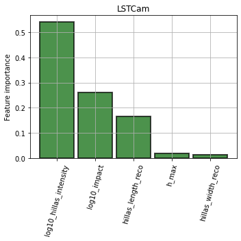
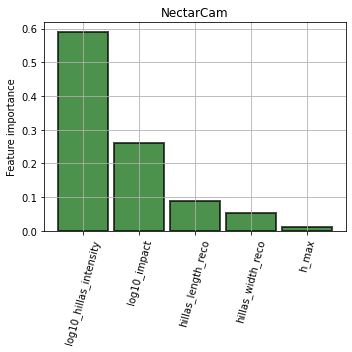
Feature importance
[15]:
for camera in cameras:
    plt.figure(figsize=(5, 5))
    ax = plt.gca()
    ax = diagnostic[camera].plot_feature_importance(
        ax,
        **{"alpha": 0.7, "edgecolor": "black", "linewidth": 2, "color": "darkgreen"}
    )
    ax.set_ylabel("Feature importance")
    ax.grid()
    plt.title(camera)
    plt.tight_layout()
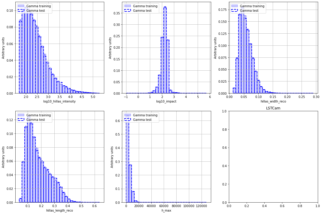
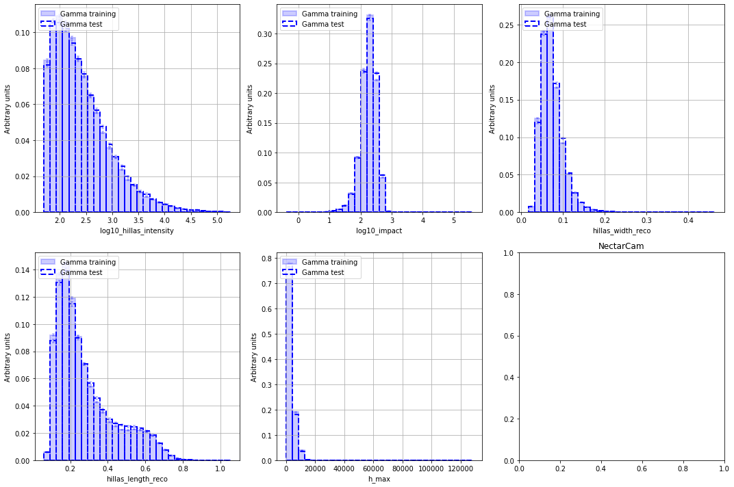
Feature distributions
[16]:
for camera in cameras:

    print("              ====================================================================================")
    print(f"                                                  {camera}                                           ")
    print("              ====================================================================================")

    fig, axes = diagnostic[camera].plot_features(
        data_list=[data[camera]["data_train"], data[camera]["data_test"]],
        nbin=30,
        hist_kwargs_list=[
            {
                "edgecolor": "blue",
                "color": "blue",
                "label": "Gamma training",
                "alpha": 0.2,
                "fill": True,
                "ls": "-",
                "lw": 2,
            },
            {
                "edgecolor": "blue",
                "color": "blue",
                "label": "Gamma test",
                "alpha": 1,
                "fill": False,
                "ls": "--",
                "lw": 2,
            },
        ],
        error_kw_list=[
            dict(ecolor="blue", lw=2, capsize=2, capthick=2, alpha=0.2),
            dict(ecolor="blue", lw=2, capsize=2, capthick=2, alpha=0.2),
        ],
        ncols=3,
    )
    plt.title(camera)
    fig.tight_layout()
              ====================================================================================
                                                  LSTCam
              ====================================================================================
              ====================================================================================
                                                  NectarCam
              ====================================================================================
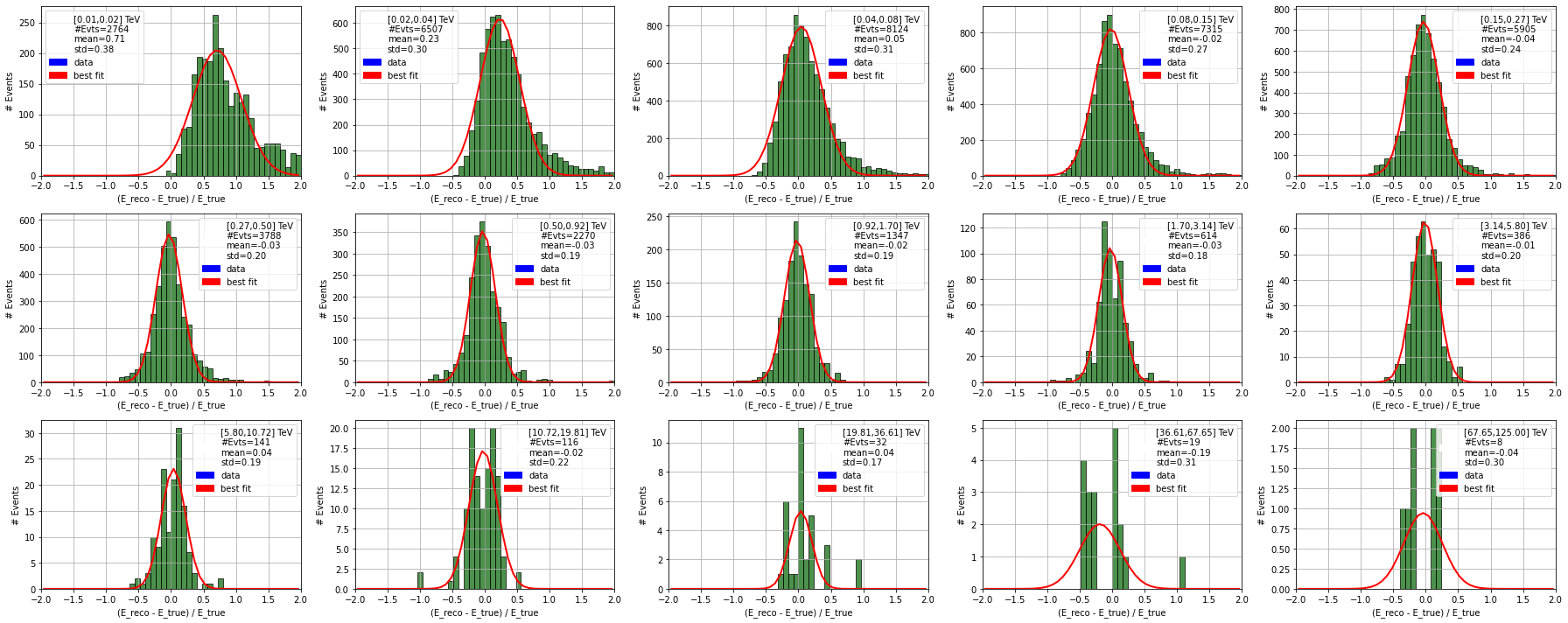
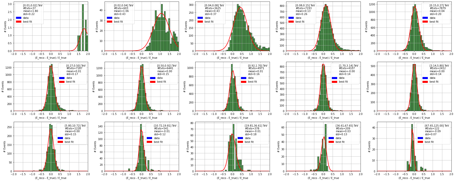
Migration distribution
[17]:
for camera in cameras:
    # Compute averaged energy
    # print("Process test sample...")

    print("              ====================================================================================")
    print(f"                                                  {camera}                                           ")
    print("              ====================================================================================")

    data_test_evt = get_evt_subarray_model_output(
        data[camera]["data_test"],
        weight_name="hillas_intensity_reco",
        keep_cols=["tel_id", "true_energy"],
        model_output_name="reco_energy_img",
        model_output_name_evt="reco_energy",
    )

    ncols = 5
    nrows = (
        int(nbins / ncols) if nbins % ncols == 0 else int((nbins + 1) / ncols)
    )
    if nrows == 0:
        nrows = 1
        ncols = 1
    fig, axes = plt.subplots(nrows=nrows, ncols=ncols, figsize=(5 * 5, 10))
    try:
        axes = axes.flatten()
    except:
        axes = [axes]

    bias = []
    resolution = []
    energy_centres = []

    for ibin in range(len(energy_edges) - 1):
        ax = axes[ibin]

        test_data = data_test_evt.query(
            "true_energy >= {} and true_energy < {}".format(
                energy_edges[ibin], energy_edges[ibin + 1]
            )
        )
        # print("Estimate energy for {} evts".format(len(test_data)))

        er = test_data["reco_energy"]
        emc = test_data["true_energy"]

        opt_hist = {
            "edgecolor": "black",
            "color": "darkgreen",
            "label": "data",
            "alpha": 0.7,
            "fill": True,
        }
        opt_fit = {"c": "red", "lw": 2, "label": "Best fit"}
        ax, fit_param, cov = diagnostic[camera].plot_resolution_distribution(
            ax=ax,
            y_true=emc,
            y_reco=er,
            nbin=50,
            fit_range=[-2, 2],
            hist_kwargs=opt_hist,
            fit_kwargs=opt_fit,
        )
        if fit_param[2] < 0:  # negative value are allowed for the fit
            fit_param[2] *= -1

        label = "[{:.2f},{:.2f}] TeV\n#Evts={}\nmean={:.2f}\nstd={:.2f}".format(
            energy_edges[ibin],
            energy_edges[ibin + 1],
            len(er),
            fit_param[1],
            fit_param[2],
        )

        ax.set_ylabel("# Events")
        ax.set_xlabel("(E_reco - E_true) / E_true")
        ax.set_xlim([-2, 2])
        ax.grid()

        evt_patch = mpatches.Patch(color="white", label=label)
        data_patch = mpatches.Patch(color="blue", label="data")
        fit_patch = mpatches.Patch(color="red", label="best fit")
        ax.legend(loc="best", handles=[evt_patch, data_patch, fit_patch])
        plt.tight_layout()

        #print(
        #    " Fit results: ({:.3f},{:.3f} TeV)".format(
        #        energy_edges[ibin], energy_edges[ibin + 1]
        #    )
        #)

        #try:
        #    print(" - A    : {:.3f} +/- {:.3f}".format(fit_param[0], cov[0][0]))
        #    print(" - mean : {:.3f} +/- {:.3f}".format(fit_param[1], cov[1][1]))
        #    print(" - std  : {:.3f} +/- {:.3f}".format(fit_param[2], cov[2][2]))
        #except:
        #    print(" ==> Problem with fit, no covariance...".format())
        #    continue

        bias.append(fit_param[1])
        resolution.append(fit_param[2])
        energy_centres.append(
            (energy_edges[ibin] + energy_edges[ibin + 1]) / 2.0
        )
    plt.show()
              ====================================================================================
                                                  LSTCam
              ====================================================================================
              ====================================================================================
                                                  NectarCam
              ====================================================================================
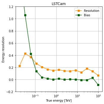
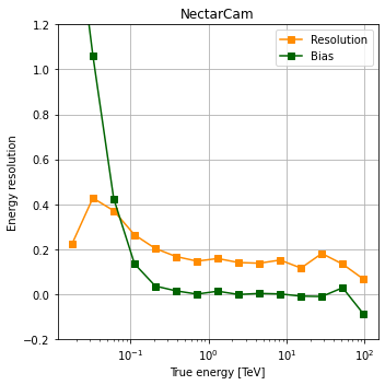
Energy resolution and bias
[18]:
for camera in cameras:

    plt.figure(figsize=(5, 5))
    ax = plt.gca()
    ax.plot(
        energy_centres,
        resolution,
        marker="s",
        color="darkorange",
        label="Resolution",
    )
    ax.plot(energy_centres, bias, marker="s", color="darkgreen", label="Bias")
    ax.set_xlabel("True energy [TeV]")
    ax.set_ylabel("Energy resolution")
    ax.set_xscale("log")
    ax.grid()
    ax.legend()
    ax.set_ylim([-0.2, 1.2])
    plt.title(camera)
    plt.tight_layout()
[ ]: