# Remove input cells at runtime (nbsphinx)
import IPython.core.display as d
d.display_html('<script>jQuery(function() {if (jQuery("body.notebook_app").length == 0) { jQuery(".input_area").toggle(); jQuery(".prompt").toggle();}});</script>', raw=True)

Particle classification (MODEL)

This notebook contains the same code as in protopipe.scripts.model_diagnostic. It should be used to test the performance of the trained model before use it to estimate the particle type of DL2 events.

In fact, what happens in a protopipe analysis is that part of the TRAINING sample is used for testing the models to get some preliminary diagnostics. This notebook shows this camera-wise preliminary diagnostics.

Settings and setup of the plots are done using the same configuration file used for training the model.

Developers

Please, if you have any contribution regarding this part, do it here and not in the relevant sections of the main code, which are now discontinued.

Table of contents

• Feature importance

• Feature distributions

• Boosted Decision Tree Error rate

• Model output

• Energy-dependent distributions

• Energy-dependent ROC curves

import gzip
import glob
from os import path

import pickle
import joblib
import yaml
import numpy as np
import pandas as pd
from scipy.optimize import curve_fit
from sklearn.metrics import auc, roc_curve

import matplotlib.pyplot as plt
import matplotlib.patches as mpatches
plt.rcParams.update({'figure.max_open_warning': 0})

def load_config(name):
    """Load YAML configuration file."""
    try:
        with open(name, "r") as stream:
            cfg = yaml.load(stream, Loader=yaml.FullLoader)
    except FileNotFoundError as e:
        print(e)
        raise
    return cfg

def load_obj(name ):
    """Load object in binary"""
    with gzip.open(name, 'rb') as f:
        return pickle.load(f)

def plot_hist(ax, data, nbin, limit, norm=False, yerr=False, hist_kwargs={}, error_kw={}):
    """Utility function to plot histogram"""
    bin_edges = np.linspace(limit[0], limit[-1], nbin + 1, True)
    y, tmp = np.histogram(data, bins=bin_edges)
    weights = np.ones_like(y)
    if norm is True:
        weights = weights / float(np.sum(y))
    if yerr is True:
        yerr = np.sqrt(y) * weights
    else:
        yerr = np.zeros(len(y))

    centers = 0.5 * (bin_edges[1:] + bin_edges[:-1])
    width = bin_edges[1:] - bin_edges[:-1]
    ax.bar(centers, y * weights, width=width, yerr=yerr, error_kw=error_kw, **hist_kwargs)

    return ax

def plot_distributions(feature_list,
                       data_list,
                       nbin=30,
                       hist_kwargs_list={},
                       error_kw_list={},
                       ncols=2):
    """Plot feature distributions for several data set. Returns list of axes."""
    n_feature = len(feature_list)
    nrows = int(n_feature / ncols) if n_feature % ncols == 0 else round((n_feature + 1) / ncols)

    fig, axes = plt.subplots(nrows=nrows, ncols=ncols, figsize=(5 * ncols, 5 * nrows))
    if nrows == 1 and ncols == 1:
        axes = [axes]
    else:
        axes = axes.flatten()

    for i, colname in enumerate(feature_list):
        ax = axes[i]

        # Range for binning
        range_min = min([data[colname].min() for data in data_list])
        range_max = max([data[colname].max() for data in data_list])
        myrange = [range_min, range_max]

        for j, data in enumerate(data_list):
            ax = plot_hist(
                ax=ax, data=data[colname], nbin=nbin, limit=myrange,
                norm=True, yerr=True,
                hist_kwargs=hist_kwargs_list[j],
                error_kw=error_kw_list[j]
            )

        ax.set_xlabel(colname)
        ax.set_ylabel('Arbitrary units')
        ax.legend(loc='upper left')
        ax.grid()
    plt.tight_layout()

    return fig, axes

def plot_roc_curve(ax, model_output, y, **kwargs):
    """Plot ROC curve for a given set of model outputs and labels"""
    fpr, tpr, _ = roc_curve(y_score=model_output, y_true=y)
    roc_auc = auc(fpr, tpr)
    label = '{} (area={:.2f})'.format(kwargs.pop('label'), roc_auc)  # Remove label
    ax.plot(fpr, tpr, label=label, **kwargs)
    return ax

def get_evt_subarray_model_output(data,
                                  weight_name=None,
                                  keep_cols=['reco_energy'],
                                  model_output_name='score_img',
                                  model_output_name_evt='score'):
    """
    Returns DataStore with keepcols + score/target columns of model at the
    level-subarray-event.

    Parameters
    ----------
    data: `~pandas.DataFrame`
        Data frame
    weight_name: `str`
        Variable name in data frame to weight events with
    keep_cols: `list`, optional
        List of variables to keep in resulting data frame
    model_output_name: `str`, optional
        Name of model output (image level)
    model_output_name: `str`, optional
        Name of averaged model output (event level)

    Returns
    --------
    data: `~pandas.DataFrame`
        Data frame
    """

    keep_cols += [model_output_name]
    keep_cols += [weight_name]
    new_data = data[keep_cols].copy(deep=True)

    new_data[model_output_name_evt] = np.zeros(len(new_data))
    new_data.set_index(["tel_id"], append=True, inplace=True)

    new_data[model_output_name_evt] = new_data.groupby(["obs_id", "event_id"]).apply(
        lambda g: np.average(g[model_output_name], weights=g[weight_name])
    )

    # Remove columns
    new_data = new_data.drop(columns=[model_output_name])

    # Remove duplicates
    new_data = new_data[~new_data.index.duplicated(keep="first")]

    return new_data

class ModelDiagnostic(object):
    """
    Base class for model diagnostics.

    Parameters
    ----------
    model: `~sklearn.base.BaseEstimator`
        Best model
    feature_name_list: list
        List of the features used to buil the model
    target_name: str
        Name of the target (e.g. score, gamaness, energy, etc.)
    """
    def __init__(self, model, feature_name_list, target_name):
        self.model = model
        self.feature_name_list = feature_name_list
        self.target_name = target_name

    def plot_feature_importance(self, ax, **kwargs):
        """
        Plot importance of features
        Parameters
        ----------
        ax: `~matplotlib.axes.Axes`
            Axis
        """
        if ax is None:
            import matplotlib.pyplot as plt
            ax = plt.gca()

        importance = self.model.feature_importances_
        importance, feature_labels = \
            zip(*sorted(zip(importance, self.feature_name_list), reverse=True))

        bin_edges = np.arange(0, len(importance)+1)
        bin_width = bin_edges[1:] - bin_edges[:-1] - 0.1

        ax.bar(bin_edges[:-1], importance, width=bin_width, **kwargs)
        ax.set_xticks(np.arange(0, len(importance)))
        ax.set_xticklabels(feature_labels, rotation=75)

        return ax

    def plot_features(self, data_list,
                      nbin=30,
                      hist_kwargs_list={},
                      error_kw_list={},
                      ncols=2):
        """
        Plot model features for different data set (e.g. training and test samples).
        Parameters
        ----------
        data_list: list
            List of data
        nbin: int
            Number of bin
        hist_kwargs_list: dict
            Dictionary with histogram options
        error_kw_list: dict
            Dictionary with error bar options
        ncols: int
            Number of columns
        """
        return plot_distributions(
            self.feature_name_list,
            data_list,
            nbin,
            hist_kwargs_list,
            error_kw_list, ncols
        )

    def add_image_model_output(self):
        raise NotImplementedError("Please Implement this method")

class ClassifierDiagnostic(ModelDiagnostic):
    """
    Class to plot several diagnostic plot for classification. Assume that positives and
    negatives are respectively labeled as 1 and 0.
    Parameters
    ----------
    model: sklearn.base.BaseEstimator
        Scikit model
    feature_name_list: list
        List of features
    model_output_name: str
        Name of output
    is_output_proba: bool
        If false, `decision_function` will be called, otherwise, predict_proba.
        In the last case we only consider the probability for signal event
    """
    def __init__(self, model, feature_name_list, target_name,
                 data_train, data_test, model_output_name='score', is_output_proba=False):
        super().__init__(model, feature_name_list, target_name)

        self.data_train = data_train
        self.data_test = data_test
        self.model_output_name = model_output_name
        self.is_output_proba = is_output_proba

        # Compute and add model output
        self.data_train = self.add_image_model_output(
            self.data_train,
            col_name=self.model_output_name
        )
        self.data_test = self.add_image_model_output(
            self.data_test,
            col_name=self.model_output_name
        )

    def add_image_model_output(self, data, col_name):
        """Add model output column"""
        if self.is_output_proba is False:
            data[col_name] = self.model.decision_function(data[self.feature_name_list])
        else:  # Interested in signal probability
            data[col_name] = self.model.predict_proba(data[self.feature_name_list])[:,1]
        return data

    def plot_image_model_output_distribution(
            self,
            cut=None,
            nbin=30,
            hist_kwargs_list=[
                {'edgecolor': 'blue', 'color': 'blue', 'label': 'Gamma training sample',
                'alpha': 0.2, 'fill': True, 'ls': '-', 'lw': 2},
                {'edgecolor': 'blue', 'color': 'blue', 'label': 'Gamma test sample',
                'alpha': 1, 'fill': False, 'ls': '--', 'lw': 2},
                {'edgecolor': 'red', 'color': 'red', 'label': 'Proton training sample',
                'alpha': 0.2, 'fill': True, 'ls': '-', 'lw': 2},
                {'edgecolor': 'red', 'color': 'red', 'label': 'Proton test sample',
                'alpha': 1, 'fill': False, 'ls': '--', 'lw': 2}
            ],
            error_kw_list=[
                dict(ecolor='blue', lw=2, capsize=3, capthick=2, alpha=0.2),
                dict(ecolor='blue', lw=2, capsize=3, capthick=2, alpha=1),
                dict(ecolor='red', lw=2, capsize=3, capthick=2, alpha=0.2),
                dict(ecolor='red', lw=2, capsize=3, capthick=2, alpha=1)
                ]
    ):
        """Plot output distribution. Need more output column"""
        if cut is not None:
            data_test = self.data_test.query(cut)
            data_train = self.data_train.query(cut)
        else:
            data_test = self.data_test
            data_train = self.data_train

        return plot_distributions(
            [self.model_output_name],
            [data_train.query('label==1'), data_test.query('label==1'),
             data_train.query('label==0'), data_test.query('label==0')],
            nbin,
            hist_kwargs_list,
            error_kw_list,
            1
        )

# Please, if you modify this notebook through a pull request empty these variables before pushing
# Note that these notebooks will show the results on the documentation!
# For this reason, if you plan to use them for your own testing, please work on a copy of this notebook

analysesDir = ""
analysisName = ""

configuration = f"{analysesDir}/{analysisName}/configs/classifier.yaml"

cfg = load_config(configuration)
model_type = cfg["General"]["model_type"]
method_name = cfg["Method"]["name"]

inDir = f"{analysesDir}/{analysisName}/estimators/gamma_hadron_classifier"
cameras = [model.split('/')[-1].split('_')[2] for model in glob.glob(f"{inDir}/{model_type}*.pkl.gz")]

data = {camera : dict.fromkeys(["model", "data_scikit", "data_train", "data_test"]) for camera in cameras}

for camera in cameras:

    data[camera]["data_scikit"] = load_obj(
                glob.glob(f"{inDir}/data_scikit_{model_type}_{method_name}_*_{camera}.pkl.gz")[0]
                )
    data[camera]["data_train"] = pd.read_pickle(
        glob.glob(f"{inDir}/data_train_{model_type}_{method_name}_*_{camera}.pkl.gz")[0]
                )
    data[camera]["data_test"] = pd.read_pickle(
        glob.glob(f"{inDir}/data_test_{model_type}_{method_name}_*_{camera}.pkl.gz")[0]
    )

    modelName = f"{model_type}_*_{camera}_{method_name}.pkl.gz"
    data[camera]["model"] = joblib.load(glob.glob(f"{inDir}/{modelName}")[0])

if cfg["Method"]["use_proba"] is True:
    ouput_model_name = "gammaness"
else:
    ouput_model_name = "score"

# Energy (both true and reconstructed)
nbins = cfg["Diagnostic"]["energy"]["nbins"]

energy_edges = np.logspace(
        np.log10(cfg["Diagnostic"]["energy"]["min"]),
        np.log10(cfg["Diagnostic"]["energy"]["max"]),
        nbins + 1,
        True,
    )

# Parameters for energy variation
cut_list = [
    "reco_energy >= {:.2f} and reco_energy <= {:.2f}".format(
        energy_edges[i], energy_edges[i + 1]
    )
    for i in range(len(energy_edges) - 1)
]

diagnostic = dict.fromkeys(cameras)
for camera in cameras:
    diagnostic[camera] = ClassifierDiagnostic(
                    model=data[camera]["model"],
                    feature_name_list=cfg["FeatureList"],
                    target_name=cfg["Method"]["target_name"],
                    data_train=data[camera]["data_train"],
                    data_test=data[camera]["data_test"],
                    model_output_name=ouput_model_name,
                    is_output_proba=cfg["Method"]["use_proba"],
                )

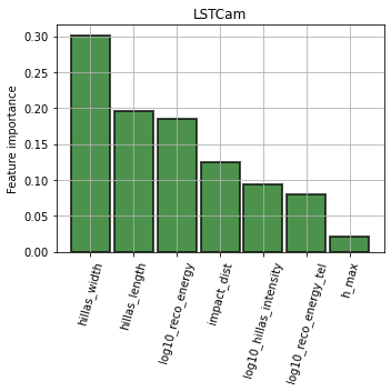
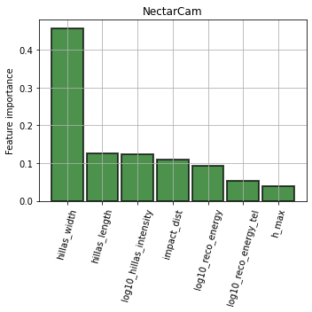
Feature importance

back to top

for camera in cameras:
    plt.figure(figsize=(5, 5))
    ax = plt.gca()
    ax = diagnostic[camera].plot_feature_importance(
        ax,
        **{"alpha": 0.7, "edgecolor": "black", "linewidth": 2, "color": "darkgreen"}
    )
    ax.set_ylabel("Feature importance")
    ax.grid()
    plt.title(camera)
    plt.tight_layout()

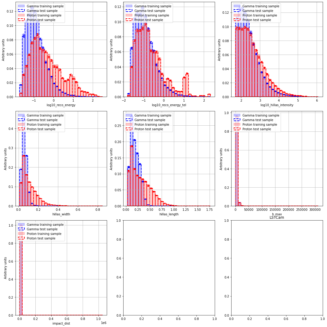
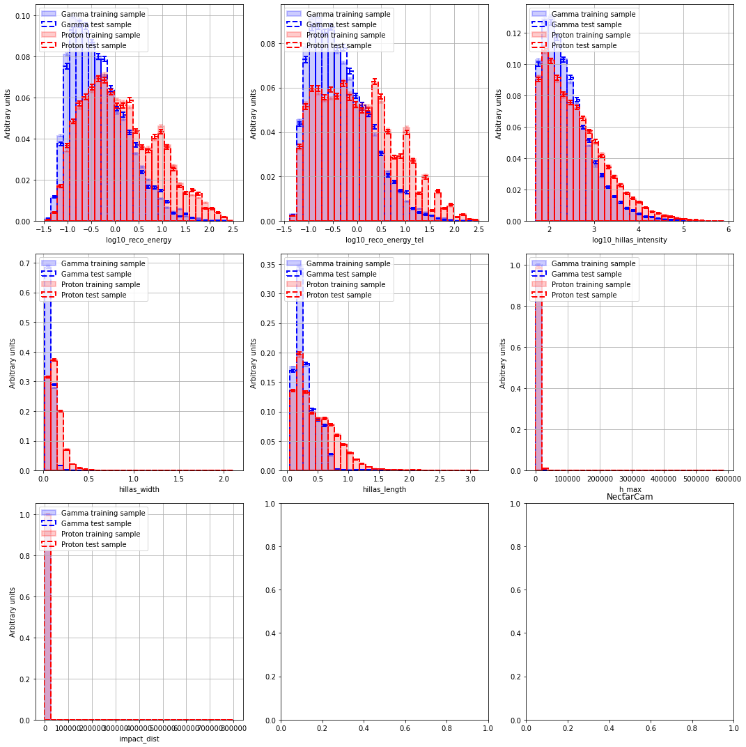
Feature distributions

back to top

for camera in cameras:

    print("              ====================================================================================")
    print(f"                                                  {camera}                                           ")
    print("              ====================================================================================")

    fig, axes = diagnostic[camera].plot_features(
                data_list=[
                    data[camera]["data_train"].query("label==1"),
                    data[camera]["data_test"].query("label==1"),
                    data[camera]["data_train"].query("label==0"),
                    data[camera]["data_test"].query("label==0"),
                ],
                nbin=30,
                hist_kwargs_list=[
                    {
                        "edgecolor": "blue",
                        "color": "blue",
                        "label": "Gamma training sample",
                        "alpha": 0.2,
                        "fill": True,
                        "ls": "-",
                        "lw": 2,
                    },
                    {
                        "edgecolor": "blue",
                        "color": "blue",
                        "label": "Gamma test sample",
                        "alpha": 1,
                        "fill": False,
                        "ls": "--",
                        "lw": 2,
                    },
                    {
                        "edgecolor": "red",
                        "color": "red",
                        "label": "Proton training sample",
                        "alpha": 0.2,
                        "fill": True,
                        "ls": "-",
                        "lw": 2,
                    },
                    {
                        "edgecolor": "red",
                        "color": "red",
                        "label": "Proton test sample",
                        "alpha": 1,
                        "fill": False,
                        "ls": "--",
                        "lw": 2,
                    },
                ],
                error_kw_list=[
                    dict(ecolor="blue", lw=2, capsize=3, capthick=2, alpha=0.2),
                    dict(ecolor="blue", lw=2, capsize=3, capthick=2, alpha=1),
                    dict(ecolor="red", lw=2, capsize=3, capthick=2, alpha=0.2),
                    dict(ecolor="red", lw=2, capsize=3, capthick=2, alpha=1),
                ],
                ncols=3,
            )
    plt.title(camera)
    #fig.tight_layout()
    plt.show()

              ====================================================================================
                                                  LSTCam
              ====================================================================================

              ====================================================================================
                                                  NectarCam
              ====================================================================================

Boosted Decision Tree Error rate

back to top

if method_name != "AdaBoostClassifier":

    print("The model is not an AdaBoostClassifier")

else:

    for camera in cameras:
        plt.figure(figsize=(5, 5))
        ax = plt.gca()
        opt = {"color": "darkgreen", "ls": "-", "lw": 2}
        BoostedDecisionTreeDiagnostic.plot_error_rate(
            ax, model, data_scikit, **opt
        )
        plt.title(camera)
        plt.tight_layout()

        plt.figure(figsize=(5, 5))
        ax = plt.gca()
        BoostedDecisionTreeDiagnostic.plot_tree_error_rate(ax, model, **opt)
        plt.title(camera)
        plt.show()

The model is not an AdaBoostClassifier

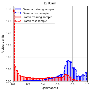
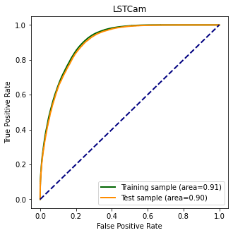
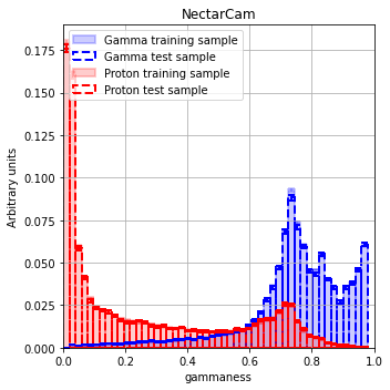
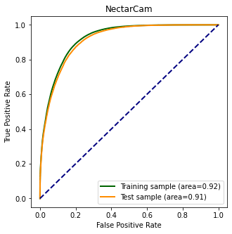
Model output

back to top

for camera in cameras:

    fig, ax = diagnostic[camera].plot_image_model_output_distribution(nbin=50)
    ax[0].set_xlim([0, 1])
    plt.title(camera)
    fig.tight_layout()

    plt.figure(figsize=(5, 5))
    ax = plt.gca()
    plot_roc_curve(
        ax,
        diagnostic[camera].data_train[diagnostic[camera].model_output_name],
        diagnostic[camera].data_train["label"],
        **dict(color="darkgreen", lw=2, label="Training sample")
    )
    plot_roc_curve(
        ax,
        data[camera]["data_test"][diagnostic[camera].model_output_name],
        diagnostic[camera].data_test["label"],
        **dict(color="darkorange", lw=2, label="Test sample")
    )
    ax.set_xlabel("False Positive Rate")
    ax.set_ylabel("True Positive Rate")
    ax.plot([0, 1], [0, 1], color="navy", lw=2, linestyle="--")
    ax.legend(loc="lower right")
    plt.title(camera)
    plt.show()

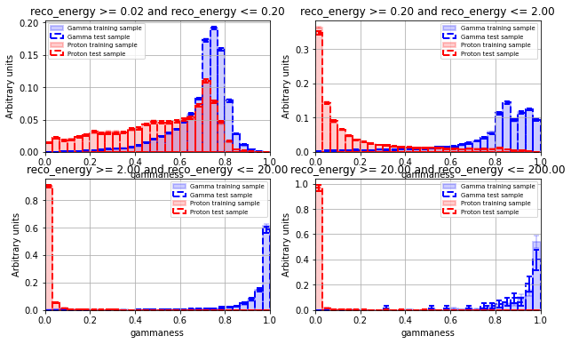
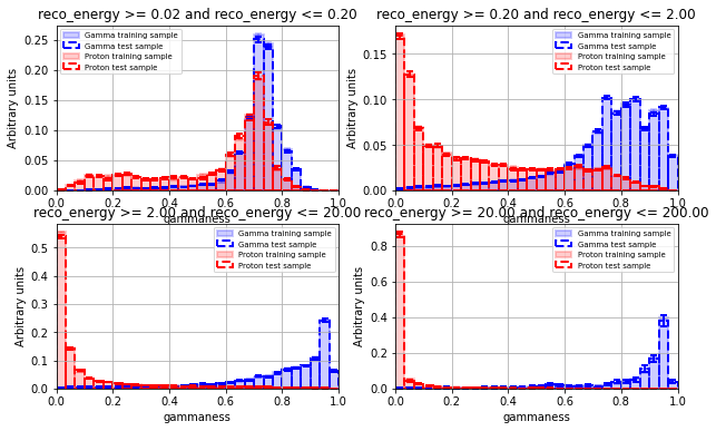
Energy-dependent distributions

back to top

hist_kwargs_list = [
    {
        "edgecolor": "blue",
        "color": "blue",
        "label": "Gamma training sample",
        "alpha": 0.2,
        "fill": True,
        "ls": "-",
        "lw": 2,
    },
    {
        "edgecolor": "blue",
        "color": "blue",
        "label": "Gamma test sample",
        "alpha": 1,
        "fill": False,
        "ls": "--",
        "lw": 2,
    },
    {
        "edgecolor": "red",
        "color": "red",
        "label": "Proton training sample",
        "alpha": 0.2,
        "fill": True,
        "ls": "-",
        "lw": 2,
    },
    {
        "edgecolor": "red",
        "color": "red",
        "label": "Proton test sample",
        "alpha": 1,
        "fill": False,
        "ls": "--",
        "lw": 2,
    },
]

error_kw_list = [
    dict(ecolor="blue", lw=2, capsize=3, capthick=2, alpha=0.2),
    dict(ecolor="blue", lw=2, capsize=3, capthick=2, alpha=1),
    dict(ecolor="red", lw=2, capsize=3, capthick=2, alpha=0.2),
    dict(ecolor="red", lw=2, capsize=3, capthick=2, alpha=1),
]

n_feature = len(cut_list)
ncols = 2
nrows = (
    int(n_feature / ncols)
    if n_feature % ncols == 0
    else int((n_feature + 1) / ncols)
)

for camera in cameras:

    print("              ====================================================================================")
    print(f"                                                  {camera}                                           ")
    print("              ====================================================================================")

    fig, axes = plt.subplots(
        nrows=nrows, ncols=ncols, figsize=(5 * ncols, 3 * nrows)
    )
    if nrows == 1 and ncols == 1:
        axes = [axes]
    else:
        axes = axes.flatten()

    data_list = [
        data[camera]["data_train"].query("label==1"),
        data[camera]["data_test"].query("label==1"),
        data[camera]["data_train"].query("label==0"),
        data[camera]["data_test"].query("label==0"),
    ]

    for i, colname in enumerate(cut_list):
        ax = axes[i]

        # Range for binning
        the_range = [0, 1]

        for j, d in enumerate(data_list):
            if len(d) == 0:
                continue

            ax = plot_hist(
                ax=ax,
                data=d.query(cut_list[i])[ouput_model_name],
                nbin=30,
                limit=the_range,
                norm=True,
                yerr=True,
                hist_kwargs=hist_kwargs_list[j],
                error_kw=error_kw_list[j],
            )

        ax.set_xlim(the_range)
        ax.set_xlabel(ouput_model_name)
        ax.set_ylabel("Arbitrary units")
        ax.legend(loc="best", fontsize="x-small")
        ax.set_title(cut_list[i])
        ax.grid()

    plt.show()

              ====================================================================================
                                                  LSTCam
              ====================================================================================

              ====================================================================================
                                                  NectarCam
              ====================================================================================

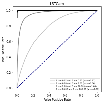
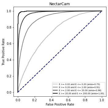
ROC curve variation on test sample

back to top

for camera in cameras:

    plt.figure(figsize=(5, 5))
    ax = plt.gca()

    color = 1.0
    step_color = 1.0 / (len(cut_list))
    for i, cut in enumerate(cut_list):
        c = color - (i + 1) * step_color

        test_data = data[camera]["data_test"].query(cut)
        if len(test_data) == 0:
            continue

        opt = dict(
            color=str(c),
            lw=2,
            label="{}".format(cut.replace("reco_energy", "E")),
        )
        plot_roc_curve(ax, test_data[ouput_model_name], test_data["label"], **opt)
    ax.plot([0, 1], [0, 1], color="navy", lw=2, linestyle="--")
    ax.set_title(camera)
    ax.set_xlabel("False Positive Rate")
    ax.set_ylabel("True Positive Rate")
    ax.legend(loc="lower right", fontsize="x-small")
    plt.tight_layout()